■【PartⅠ Law for Translating Music into Painting ・・・ Here is the Python program】 I have finally unveiled and publicly released This Law , ending six years of secrecy surrounding it. Here is the Python program that demonstrates and verifies the law.

 I am Masahiko Yokota, a contemporary artist living in Sapporo, Japan.
Today, I have finally lifted the six-year seal of secrecy on the “Physical Laws for Converting Musical Scores into Paintings,” which I had kept confidential for six years, except for publicly explaining the entire theory to Yutetsu Yamamoto, representative of Tokyo Gallery, at Tokyo Gallery in Ginza.
The reasons for making it public are as follows.
- New theories and discoveries in physics and other scientific fields cannot be patented.
- Over the six years, I have produced and accumulated more than ten large-scale pastel paintings using these laws.
- Simply saying “I discovered it” often failed to convince people in the end..
For these reasons, I have now made the evidence public together with the complete contents of the laws!
Please determine for yourself whether these laws are true by examining the programs below and the statements made by various musicians and music professionals!
Can “music,” an art of hearing, be transformed into “painting,” an art of seeing?
The answer “Yes, it can” to this question, for the first time in the history of art, is what these laws represent.
This time, I created and executed a Python program to verify this theory, and the results were successfully visualized exactly as predicted by the theory, thereby demonstrating the validity of these laws.
Now, I will reveal the complete picture of these laws!
Four Laws for Turning Musical Scores into Paintings
① The Musical Scale Corresponds to the Spectrum of Light (the Colors of the Rainbow)
The seven notes of the Do-Re-Mi-Fa-So-La-Ti-Do scale correspond completely to the wavelengths (colors) of light.  Do (C) = Red
Re (D) = Orange
Mi (E) = Yellow
Fa (F) = Yellow-green
So (G) = Green
La (A) = Blue
Ti (B) = Purple
Because colors become higher in frequency as they move upward, we can think of each successive octave as becoming brighter!
◆I did not know this until I completed my theory, but in fact, a person named Maryon proposed almost exactly the same idea as early as 1919. However, the theoretical development did not progress beyond that point..
② The Tonic Note of Music Becomes the Dominant Color of the Painting — The Main Color Covering the Canvas
From this point onward, the theory is something that Maryon and previous researchers had not discovered.。

Tonal music means that if a piece begins with Do and ends with Do, it is in C major.
If it begins with Mi, it becomes D major.
A piece that begins with the note between Do and Mi becomes D minor.
Major notes such as Do-Re-Mi sound “bright,” while the individual notes corresponding to the black keys on a piano, which lie between the major notes, sound dark.
The tonic note therefore determines the overall character and atmosphere of the piece. Is it a bright-sounding piece or a dark-sounding piece?
In other words, it governs the entire piece.
In painting, the color corresponding to each note becomes the color that dominates the entire canvas.
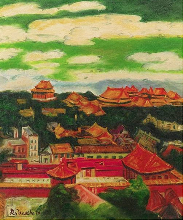
Therefore, when C major is translated into a painting, red becomes the dominant color of the canvas, as in Ryuzaburo Umehara's “Sakurajima — Red” below.
Conversely, “Sakurajima — Blue” is, yes, B major.
Without thinking in this way, there is no way to explain why the overall atmosphere of music is determined by keys such as C major and A minor.
My theory also explains perfectly the role of the principal color in painting, does it not?
 Atonal music began with Schoenberg's twelve-tone serial music. If so, as you can see by running the chord-drawing program below,
minor keys become “dull intermediate colors” between red and vermilion, and between blue and purple.
In other words, they are not pure colors. They can be thought of as muddy intermediate colors.
This creates a sad, twilight-like painting.
There is a remarkable anecdote that while the Kandinsky couple and the Schoenberg couple were talking together in a room, Schoenberg's wife Nina said that “Picasso's work (The Dream (The Sleeping Woman in a Red Chair)) and photographs are the realization of twelve-tone music in painting!” This is a profound observation because the work has no basic color dominating the canvas.
④ The Relationship Between Pitch and Painting
 Melody is arranged on the canvas as “time (X-axis)” and “height (Y-axis).”
◆Time (duration of a note):
One beat (a quarter note) is represented by one “square (□).” For example, a note held for three beats is displayed as three squares arranged horizontally. The squares representing successive notes are connected by lines to show their continuity.
◆Height (pitch):
The vertical Y-axis becomes like the floors of a building. The first floor is Do, the second floor is Re, the third floor is Mi, and so on, forming a height like a totem pole across the seven-note scale.
◆A sound has both color = timbre and pitch.
As you know, the higher the pitch, the higher its frequency.
For example, if we think of a trumpet, as Kandinsky pointed out in works such as “Concerning the Spiritual in Art,” the sound of a trumpet can be heard as a metallic sound resembling the yellow or gold that we visually associate with it, can't it?
This also has a pitch.
If that is the case, then when translating it into painting, the lower part of the canvas should be darker — that is, lower in frequency as a color — while moving upward should make it whiter and higher in frequency.
Remarkably, this is the same as nature, isn't it? It becomes a relationship between heaven and earth.
If you cannot perceive the law for replacing timbre and pitch with their equivalents in painting, you understand that colors become higher in frequency as they approach blue, while greater height also means higher frequency. Then you become confused about how to apply this when translating music into painting, and this is where you inevitably give up, isn't it?
How Should We Think About Rhythm?
When creating popular music, back when I was at university and demonstrated my own composition on NHK-FM, I first created the rhythm with a metronome-like sound, then added the chords using a keyboard, and finally placed the melody over the rhythm and chord progression, completing the piece. It seems that Led Zeppelin also used this method, making it one of the most orthodox methods of composition, wouldn't you say?
In popular music, the composer or a lyricist then adds lyrics, and the song is complete.
This underlying, fundamental rhythm is handled by instruments such as the bass and drums.
Below is a painting of Charlie Watts's drum performance in The Rolling Stones' “Satisfaction.”
Since the melody is the theme and image of the song, the differences in note lengths as the melody is successively drawn toward the right become the rhythm!
This is where previous paintings differ from tonal music and popular music: flat paintings by Matisse and Picasso do not contain this rhythm.
They express rhythm only slightly through distortions of lines, so they do not convey the dynamic energy and vitality of rock music, do they?
How Can Chords Be Visualized?
Representative chords such as Do-Re-Mi and Re-Fa-La can easily be visualized as follows through the one-to-one correspondence between notes and the spectrum, can't they?
The national painter Ryuzaburo Umehara was the artist who skillfully used these chords in his paintings.
I will explain the details of this in the next post.
The chord-visualization program is shown below.

Examples of Paintings in Which Color Chords Are Actually Used
According to this law, the C major chord, Do-Mi-So, corresponds to “red, yellow, green.”
The Dm (D minor) chord, Re-Fa-La, corresponds to “vermilion, yellow-green, blue,” doesn't it?
Take a look at this work. It is Ryuzaburo Umehara's painting of Mount Fuji. When it was first exhibited, it made such an impact on the public that a newspaper praised it as “a masterpiece like a grand slam home run with the bases loaded!”
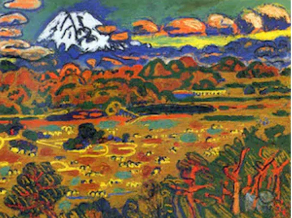
At the foot of Mount Fuji, the small mountain range consists of “red and green, with yellow in the clouds above,” while the plain below the mountain range is also yellow, isn't it?
See? Isn't this a C major chord?
●What I want you to notice is that the clouds are vermilion, with additional “yellow.” This yellow makes the entire painting stand out particularly strongly.
This further enhances the harmony of the C major chord, doesn't it?
Furthermore, there is vermilion in both the mountain range and the plain. The clouds are also vermilion, with yellow-green beneath them, and the mountain range below that is blue.
See? It is a magnificent Dm chord.
Umehara may have vaguely sensed the relationship between colors and the spectrum, but perhaps he was not consciously aware of it.
But at the very least, he must have clearly recognized as a law the highly emotional and harmonious effect produced by the theory of “three-color chords,” that is, the established combinations of three colors.
Because this established principle could not be discerned, other painters who wanted to create works capable of producing the same emotional impact as Umehara's were unable to do so, no matter how hard they tried.
I was one of them.
Programs Based on This Law
I have programmed this law as follows.
First, when I visualized Ryuichi Sakamoto's “The Last Emperor,” the Forbidden City, the landscapes of Guilin, and the associated imagery appeared exactly as I had anticipated.
What does this mean? Composers do not compose simply by having sounds float through their minds. They compose while imagining specific landscapes and scenes..
This is precisely why lyricists such as Takashi Matsumoto can place lyrics over a melody that perfectly match the imagery evoked by the music.
Let me say it again.
“Popular songs and other tonal music are not abstract art!”
“The idea that all music is abstract art, like abstract painting, is incorrect!”
A member of a certain classical orchestra told me, regarding this opinion of mine, “I myself, and classical performers such as orchestra members, had all vaguely but clearly understood that this was probably the case!”
Don't you think so too?
In other words, popular music and other tonal music are ‘figurative paintings’!
Until now, abstract painters have assumed that “all music is abstract art” and, based on that assumption, have placed dots, lines, planes, colors, and textures according to “sensation and impression.”
In other words, most abstract painters in the world could be described as “abstract impressionists” or “abstract sensualists.”
They place dots, lines, planes, and colors on the canvas somewhat intuitively.
But there is no “necessity,” a word that was one of Kandinsky's habitual expressions.
Instead of necessity, there is “something like this.”
Therefore, many abstract painters must have suffered tremendously from the unavoidable loss and lack of the explanatory power of concrete objects that lyrics possess.
They simply cannot “explain or express at all” concrete objects, landscapes, flowers, trees, people, or their distinctive individual characteristics, can they?
This is an extremely painful experience. After all, it means that they cannot adequately communicate to the viewer what they want to say or convey.
However, once we realize that tonal music — the pop music, popular songs, and classical music such as Bach that we normally hear — is music that begins with a tonic such as C major or A minor, and that it is figurative painting, the cause of and solution to this unbearable restriction on expression becomes visible.
Then, yes. The assumptions held by many abstract painters that “music is abstract,” and that “painting and music can never be integrated because the physical, medical, and physiological laws such as frequency are completely different,” turn out to be mistaken stereotypes. It becomes clear that the expressive theories and methods forming the foundation of their own works are extremely poor, rough, limited, and blurred.
Isn't this a Copernican revolution — a discovery that overturns the conventional wisdom of art history like turning the entire table upside down?
Therefore, this time I created a Python program that draws images according to this theory, serving as a demonstration of the theory.
Here it is.
Now, exactly according to the established principle that innovation is “the act of discerning a common law among things that had previously been regarded as completely different and unrelated, and then combining them,” painting and music have, for the first time in the history of art and the history of music, been connected and made mutually translatable.
Sample Program
Please copy and paste this program into the IDLE window and run it.
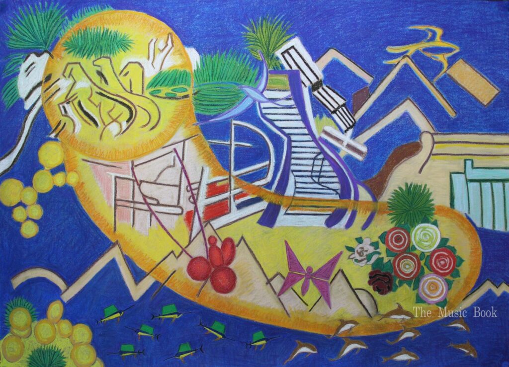
The execution result will be the same as the header image on this page.
① IDLE can be installed here.
② Launching IDLE
◆For Windows, type “IDLE” into the search box at the bottom of the screen and press Enter. 
◆For Mac, please refer to the IDLE installation page above.
② How to Run the Program
- Launch the Python development environment “IDLE,” which comes standard with Python.
- From the menu at the top of the screen, click “File” → “New File” to open a new blank window.
- Copy and paste the entire program (code) above into the window that opens.
- From the menu, click “Run” → “Run Module” (or press the F5 key on the keyboard).
- A message box saying “Source Must Be saved・・・・ Ok キャンセル” will appear. Click Ok, then enter any filename you like on the next screen and click the “保存(S)” button.
After waiting for a while, a new window will open and a visualization graph of “Do-Re-Mi Song,” based on the theory, will be drawn! Please experience for yourself the moment when music is transformed into painting.
◆Ryuichi Sakamoto: Translating the Musical Score of the Main Theme from The Last Emperor into a Painting
The music is here!
import matplotlib.pyplot as plt
import matplotlib.patches as patches
from matplotlib import colors

# ---------------------------------------------------------
# 1. 音楽データの定義(坂本龍一:ラストエンペラー メインテーマ)
# ---------------------------------------------------------
melody = [
    # 【Aメロ】
    (5, 1, 3), (6, 1, 1), (0, 2, 2), (1, 2, 2), (2, 2, 4),
    (0, 2, 2), (5, 1, 2), (4, 1, 2), (5, 1, 4),
    # 【Bメロ】
    (5, 1, 2), (0, 2, 2), (1, 2, 2), (2, 2, 2), (4, 2, 2),
    (2, 2, 4), (1, 2, 2), (0, 2, 2), (5, 1, 6),
]

# ---------------------------------------------------------
# 2. 法則に基づく色の定義
# ---------------------------------------------------------
base_colors = {
    0: '#FF0000', 1: '#FFA500', 2: '#FFFF00', 3: '#9ACD32',
    4: '#008000', 5: '#0000FF', 6: '#800080'
}

bg_colors = {
    0: '#FF76C2', 1: '#FFA376', 2: '#FFE276', 3: '#C2FF76',
    4: '#76FFC2', 5: '#76C2FF', 6: '#C276FF' # 「ラ」主調の青系背景
}

def get_color(pitch_class, octave):
    """オクターブが上がると色を明るくする関数"""
    base_rgb = colors.to_rgb(base_colors[pitch_class])
    if octave <= 1:
        return base_rgb
    else:
        factor = 1.0 - (0.5 ** (octave - 1))
        return [c + (1.0 - c) * factor for c in base_rgb]

# ---------------------------------------------------------
# 3. 描画キャンバスと背景色の設定
# ---------------------------------------------------------
fig, ax = plt.subplots(figsize=(16, 8))

# 最初の音(ラ)に基づき、青系の背景に設定
first_pitch = melody[0][0]
ax.set_facecolor(bg_colors[first_pitch])

current_x = 0
square_corners = [] # 全ての正方形の左下と右下の座標を記録するリスト

# ---------------------------------------------------------
# 4. 白大理石の基壇(漢白玉の台座)
# ---------------------------------------------------------
ax.add_patch(patches.Rectangle((0, 0), 100, 0.4, facecolor='#E0E0E0', edgecolor='#CCCCCC', zorder=1))
ax.add_patch(patches.Rectangle((0, 0.4), 100, 0.3, facecolor='#ECECEC', edgecolor='#DDDDDD', zorder=1))
ax.add_patch(patches.Rectangle((0, 0.7), 100, 0.3, facecolor='#F5F5F5', edgecolor='#EEEEEE', zorder=1))

# ---------------------------------------------------------
# 5. 音符(正方形)の配置
# ---------------------------------------------------------
for note in melody:
    pitch_class, octave, duration = note

    y = pitch_class + 1 + (octave - 1) * 7
    note_color = get_color(pitch_class, octave)

    # 指定された長さ分、正方形を並べる
    for i in range(duration):
        sq_x = current_x + i + 0.05
        sq_y = y - 0.45

        # この正方形の左下(bl)と右下(br)の座標を記録
        bl = (sq_x, sq_y)
        br = (sq_x + 0.9, sq_y)
        square_corners.append({'bl': bl, 'br': br})

        rect = patches.Rectangle((sq_x, sq_y), 0.9, 0.9,
                                 facecolor=note_color, edgecolor='black', linewidth=1.2, zorder=4)
        ax.add_patch(rect)

    current_x += duration

# ---------------------------------------------------------
# 6. 前の□の右下から、次の□の左下へ線を繋ぐ
# ---------------------------------------------------------
for i in range(len(square_corners) - 1):
    prev_br_x, prev_br_y = square_corners[i]['br']  # 前の□の右下
    next_bl_x, next_bl_y = square_corners[i+1]['bl'] # 次の□の左下

    # 薄い黒色(グレー)でシンプルに結ぶ
    ax.plot([prev_br_x, next_bl_x], [prev_br_y, next_bl_y], color='#555555', linewidth=1.5, zorder=3)

# ---------------------------------------------------------
# 7. 見た目の調整と出力
# ---------------------------------------------------------
ax.set_xlim(0, current_x)
ax.set_ylim(0, 15)

ax.set_yticks(range(1, 15))
yticklabels = ['1F: C(ド)', '2F: D(レ)', '3F: E(ミ)', '4F: F(ファ)', '5F: G(ソ)', '6F: A(ラ)', '7F: B(シ)',
               '8F: C(ド高)', '9F: D(レ高)', '10F: E(ミ高)', '11F: F(ファ高)', '12F: G(ソ高)', '13F: A(ラ高)', '14F: B(シ高)']
ax.set_yticklabels(yticklabels)

ax.set_xlabel("Time (Beats)")
ax.set_title("The Last Emperor - Music Art")

plt.grid(True, which='both', axis='y', linestyle='--', alpha=0.5, color='white', zorder=1)
plt.tight_layout()
plt.show()
Eiichi Ohtaki — A Canary Island — Main Melody Section
◆The music is here!
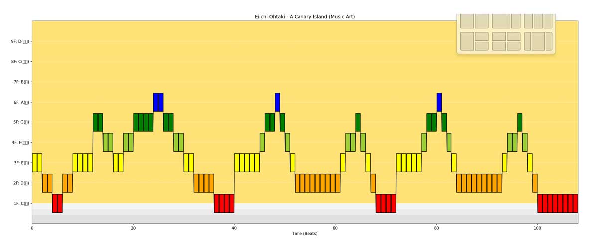
import matplotlib.pyplot as plt
import matplotlib.patches as patches
from matplotlib import colors

# ---------------------------------------------------------
# 1. 音楽データの定義(大瀧詠一:カナリア諸島にて)
# ---------------------------------------------------------
melody = [
    # 【イントロ】(南国の風を感じるストリングス風の波打つメロディ)
    (2, 1, 2), (1, 1, 2), (0, 1, 2), (1, 1, 2), (2, 1, 4),
    (4, 1, 2), (3, 1, 2), (2, 1, 2), (3, 1, 2), (4, 1, 4),
    (5, 1, 2), (4, 1, 2), (3, 1, 2), (2, 1, 2), (1, 1, 4),
    (0, 1, 4),

    # 【Aメロ】♪薄く切ったオレンジを アイスティーに浮かべて
    (2, 1, 1), (2, 1, 1), (2, 1, 2), # う・す・く
    (2, 1, 1), (3, 1, 1), (4, 1, 2), # きっ・た
    (5, 1, 1), (4, 1, 1), (3, 1, 1), (2, 1, 1), (1, 1, 4), # お・れ・ん・じ・を
    (1, 1, 1), (1, 1, 1), (1, 1, 2), # あ・い・す
    (1, 1, 1), (2, 1, 1), (3, 1, 2), # てぃ・に
    (4, 1, 1), (3, 1, 1), (2, 1, 1), (1, 1, 1), (0, 1, 4), # う・か・べ・て

    # 【Aメロ続き】♪海辺のバルコニーで 空の色を眺める
    (2, 1, 1), (2, 1, 1), (2, 1, 2), # う・み・べ
    (2, 1, 1), (3, 1, 1), (4, 1, 2), # の・
    (5, 1, 1), (4, 1, 1), (3, 1, 1), (2, 1, 1), (1, 1, 4), # ば・る・こ・に・で
    (1, 1, 1), (1, 1, 1), (1, 1, 2), # そ・ら・の
    (1, 1, 1), (2, 1, 1), (3, 1, 2), # い・ろ・
    (4, 1, 1), (3, 1, 1), (2, 1, 1), (1, 1, 1), (0, 1, 8), # な・が・め・るーー
]

# ---------------------------------------------------------
# 2. 法則に基づく色の定義
# ---------------------------------------------------------
base_colors = {
    0: '#FF0000', 1: '#FFA500', 2: '#FFFF00', 3: '#9ACD32',
    4: '#008000', 5: '#0000FF', 6: '#800080'
}

bg_colors = {
    0: '#FF76C2', 1: '#FFA376', 2: '#FFE276', 3: '#C2FF76',
    4: '#76FFC2', 5: '#76C2FF', 6: '#C276FF'
}

def get_color(pitch_class, octave):
    """オクターブが上がると色を明るくする関数"""
    base_rgb = colors.to_rgb(base_colors[pitch_class])
    if octave <= 1:
        return base_rgb
    else:
        factor = 1.0 - (0.5 ** (octave - 1))
        return [c + (1.0 - c) * factor for c in base_rgb]

# ---------------------------------------------------------
# 3. 描画キャンバスと背景色の設定
# ---------------------------------------------------------
fig, ax = plt.subplots(figsize=(20, 8)) # 曲が少し長いため横幅を広げました

# 最初の音(ミ)に基づき、背景色が自動で「カナリアイエロー(#FFE276)」に設定されます
first_pitch = melody[0][0]
ax.set_facecolor(bg_colors[first_pitch])

current_x = 0
square_corners = [] # 全ての正方形の左下と右下の座標を記録するリスト

# ---------------------------------------------------------
# 4. 白いテラスの基壇(海辺のリゾートをイメージした白い台座)
# ---------------------------------------------------------
ax.add_patch(patches.Rectangle((0, 0), 150, 0.4, facecolor='#E0E0E0', edgecolor='#CCCCCC', zorder=1))
ax.add_patch(patches.Rectangle((0, 0.4), 150, 0.3, facecolor='#ECECEC', edgecolor='#DDDDDD', zorder=1))
ax.add_patch(patches.Rectangle((0, 0.7), 150, 0.3, facecolor='#F5F5F5', edgecolor='#EEEEEE', zorder=1))

# ---------------------------------------------------------
# 5. 音符(正方形)の配置
# ---------------------------------------------------------
for note in melody:
    pitch_class, octave, duration = note

    y = pitch_class + 1 + (octave - 1) * 7
    note_color = get_color(pitch_class, octave)

    for i in range(duration):
        sq_x = current_x + i + 0.05
        sq_y = y - 0.45

        # この正方形の左下(bl)と右下(br)の座標を記録
        bl = (sq_x, sq_y)
        br = (sq_x + 0.9, sq_y)
        square_corners.append({'bl': bl, 'br': br})

        rect = patches.Rectangle((sq_x, sq_y), 0.9, 0.9,
                                 facecolor=note_color, edgecolor='black', linewidth=1.2, zorder=4)
        ax.add_patch(rect)

    current_x += duration

# ---------------------------------------------------------
# 6. 前の□の右下から、次の□の左下へ線を繋ぐ
# ---------------------------------------------------------
for i in range(len(square_corners) - 1):
    prev_br_x, prev_br_y = square_corners[i]['br']  # 前の□の右下
    next_bl_x, next_bl_y = square_corners[i+1]['bl'] # 次の□の左下

    # 薄い黒色(グレー)でシンプルに結ぶ
    ax.plot([prev_br_x, next_bl_x], [prev_br_y, next_bl_y], color='#555555', linewidth=1.5, zorder=3)

# ---------------------------------------------------------
# 7. 見た目の調整と出力
# ---------------------------------------------------------
ax.set_xlim(0, current_x)
ax.set_ylim(0, 10) # メロディの最高音に合わせて余白を調整

ax.set_yticks(range(1, 10))
yticklabels = ['1F: C(ド)', '2F: D(レ)', '3F: E(ミ)', '4F: F(ファ)', '5F: G(ソ)', '6F: A(ラ)', '7F: B(シ)',
               '8F: C(ド高)', '9F: D(レ高)']
ax.set_yticklabels(yticklabels)

ax.set_xlabel("Time (Beats)")
ax.set_title("Eiichi Ohtaki - A Canary Island (Music Art)")

plt.grid(True, which='both', axis='y', linestyle='--', alpha=0.5, color='white', zorder=1)
plt.tight_layout()
plt.show()
A Canary Island — Opening Intro Section
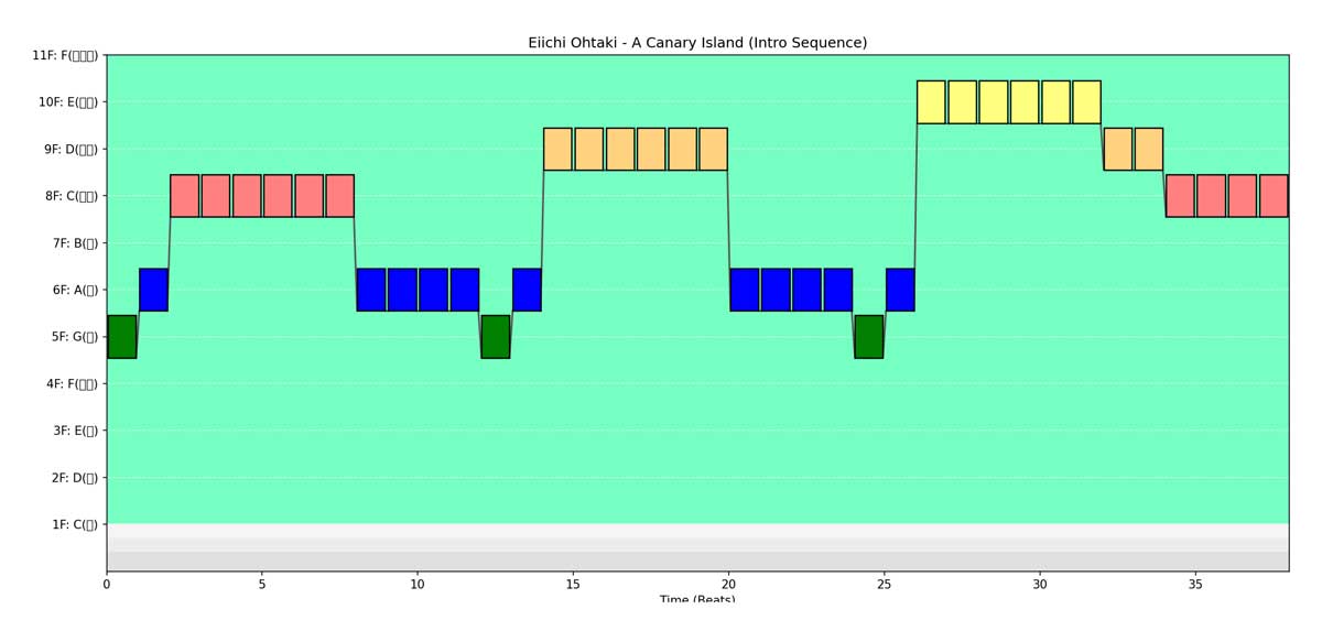
This time, I had the program visualize only the string-instrument introduction. The music is here.
import matplotlib.pyplot as plt
import matplotlib.patches as patches
from matplotlib import colors

# ---------------------------------------------------------
# 1. 音楽データの定義(大瀧詠一:カナリア諸島にて - イントロのみ)
# 「ダタダ~~ン、ダ~~ン🎵」のフレーズをブロックの長短で忠実に再現
# ---------------------------------------------------------
melody = [
    # 1回目:ダタダ~~ン(高)、ダ~~ン🎵 (ソ・ラ・ド高ーー、ラーー)
    (4, 1, 1), (5, 1, 1), (0, 2, 6), (5, 1, 4),

    # 2回目:ダタダ~~ン(高)、ダ~~ン🎵 (ソ・ラ・レ高ーー、ラーー)
    (4, 1, 1), (5, 1, 1), (1, 2, 6), (5, 1, 4),

    # 3回目:ダタダ~~ン(最高音)、ダ~~ン🎵 (ソ・ラ・ミ高ーー、レ高・ド高ー)
    (4, 1, 1), (5, 1, 1), (2, 2, 6), (1, 2, 2), (0, 2, 4),
]

# ---------------------------------------------------------
# 2. 法則に基づく色の定義(元のスペクトルに復元)
# ---------------------------------------------------------
base_colors = {
    0: '#FF0000', # ド (C): 赤
    1: '#FFA500', # レ (D): オレンジ
    2: '#FFFF00', # ミ (E): 黄色
    3: '#9ACD32', # ファ (F): 黄緑
    4: '#008000', # ソ (G): 緑
    5: '#0000FF', # ラ (A): 青
    6: '#800080'  # シ (B): 紫
}

bg_colors = {
    0: '#FF76C2', # ド (C): 薄い赤
    1: '#FFA376', # レ (D): 薄いオレンジ
    2: '#FFE276', # ミ (E): 薄い黄色
    3: '#C2FF76', # ファ (F): 薄い黄緑
    4: '#76FFC2', # ソ (G): 薄い緑(今回の主調色:リゾートグリーン)
    5: '#76C2FF', # ラ (A): 薄い青
    6: '#C276FF'  # シ (B): 薄い紫
}

def get_color(pitch_class, octave):
    """オクターブが上がると色を明るくする関数"""
    base_rgb = colors.to_rgb(base_colors[pitch_class])
    if octave <= 1:
        return base_rgb
    else:
        factor = 1.0 - (0.5 ** (octave - 1))
        return [c + (1.0 - c) * factor for c in base_rgb]

# ---------------------------------------------------------
# 3. 描画キャンバスと背景色の設定
# ---------------------------------------------------------
fig, ax = plt.subplots(figsize=(15, 7))

# 最初の音(ソ)に基づき、背景色が自動で「薄い緑(#76FFC2)」に設定されます
first_pitch = melody[0][0]
ax.set_facecolor(bg_colors[first_pitch])

current_x = 0
square_corners = []

# ---------------------------------------------------------
# 4. 白いテラスの基壇
# ---------------------------------------------------------
ax.add_patch(patches.Rectangle((0, 0), 100, 0.4, facecolor='#E0E0E0', edgecolor='#CCCCCC', zorder=1))
ax.add_patch(patches.Rectangle((0, 0.4), 100, 0.3, facecolor='#ECECEC', edgecolor='#DDDDDD', zorder=1))
ax.add_patch(patches.Rectangle((0, 0.7), 100, 0.3, facecolor='#F5F5F5', edgecolor='#EEEEEE', zorder=1))

# ---------------------------------------------------------
# 5. 音符(正方形)の配置
# ---------------------------------------------------------
for note in melody:
    pitch_class, octave, duration = note

    y = pitch_class + 1 + (octave - 1) * 7
    note_color = get_color(pitch_class, octave)

    for i in range(duration):
        sq_x = current_x + i + 0.05
        sq_y = y - 0.45

        bl = (sq_x, sq_y)
        br = (sq_x + 0.9, sq_y)
        square_corners.append({'bl': bl, 'br': br})

        rect = patches.Rectangle((sq_x, sq_y), 0.9, 0.9,
                                 facecolor=note_color, edgecolor='black', linewidth=1.2, zorder=4)
        ax.add_patch(rect)

    current_x += duration

# ---------------------------------------------------------
# 6. 前の□の右下から、次の□の左下へ線を繋ぐ
# ---------------------------------------------------------
for i in range(len(square_corners) - 1):
    prev_br_x, prev_br_y = square_corners[i]['br']
    next_bl_x, next_bl_y = square_corners[i+1]['bl']

    # 薄い黒色(グレー)でシンプルに結ぶ
    ax.plot([prev_br_x, next_bl_x], [prev_br_y, next_bl_y], color='#555555', linewidth=1.5, zorder=3)

# ---------------------------------------------------------
# 7. 見た目の調整と出力
# ---------------------------------------------------------
ax.set_xlim(0, current_x)
ax.set_ylim(0, 11)

ax.set_yticks(range(1, 12))
yticklabels = ['1F: C(ド)', '2F: D(レ)', '3F: E(ミ)', '4F: F(ファ)', '5F: G(ソ)', '6F: A(ラ)', '7F: B(シ)',
               '8F: C(ド高)', '9F: D(レ高)', '10F: E(ミ高)', '11F: F(ファ高)']
ax.set_yticklabels(yticklabels)

ax.set_xlabel("Time (Beats)")
ax.set_title("Eiichi Ohtaki - A Canary Island (Intro Sequence)")

plt.grid(True, which='both', axis='y', linestyle='--', alpha=0.5, color='white', zorder=1)
plt.tight_layout()
plt.show()
Visualization of the Main Chords of Classical Music
◆First, “C major” as a world = the scale
The C-major scale is, as everyone knows,
**Do-Re-Mi-Fa-So-La-Ti-Do**
These seven notes can be combined in groups of three to form the basic triads.
For example,
**Do-Mi-So**
played simultaneously forms the chord “C.”
C is the “center” of the music in C major.
Even if the music travels somewhere else, when it returns to C at the end, it feels like “coming home.”
This is the **tonic chord (I)**.
These are the representative chords of classical music.
| Roman Numeral | Chord | Notes | Basic Function |
|---|---|---|---|
| Ⅰ | C | Do-Mi-So | Stability / Center |
| Ⅱ | Dm | Re-Fa-La | Preparation to move forward |
| Ⅳ | F | Fa-La-Do | Moving away from the center |
| Ⅴ | G | So-Ti-Re | Creates a desire to return to C |
| Ⅴ7 | G7 | So-Ti-Re-Fa | Strong tension |
| Ⅶ° | Bdim | Ti-Re-Fa | Highly unstable |
Now, here is the program for visualizing the representative chords of classical music.
Here is the execution result.
import matplotlib.pyplot as plt
import matplotlib.patches as patches
from matplotlib import colors

# ---------------------------------------------------------
# 1. クラシック音楽(Cメジャー調)の代表的な機能和音の定義
# 形式: (和声記号と機能, コード名, 構成音)
# ---------------------------------------------------------
classic_chords = [
    ("Ⅰ\n(Tonic)", "C", [(0, 1), (2, 1), (4, 1)]),            # 主和音:安定
    ("Ⅳ\n(Subdominant)", "F", [(3, 1), (5, 1), (0, 2)]),       # 下属和音:少し動く
    ("Ⅴ\n(Dominant)", "G", [(4, 1), (6, 1), (1, 2)]),           # 属和音:緊張
    ("Ⅴ7\n(Dominant 7th)", "G7", [(4, 1), (6, 1), (1, 2), (3, 2)]), # 属七の和音:強い緊張
    ("Ⅱ\n(Supertonic)", "Dm", [(1, 1), (3, 1), (5, 1)]),        # Ⅱ度の和音(Ⅳの代理)
    ("Ⅶ°\n(Diminished)", "Bdim", [(6, 1), (1, 2), (3, 2)]),       # 減三和音:不安定
]

# カデンツ(和音の進行)のデモンストレーション用(Ⅴ7 -> Ⅰ)
cadence = [
    ("Ⅴ7 (Tension)", "G7", [(4, 1), (6, 1), (1, 2), (3, 2)]),
    ("Ⅰ (Resolution)", "C", [(0, 1), (2, 1), (4, 1)])
]

# ---------------------------------------------------------
# 2. 法則に基づく色の定義
# ---------------------------------------------------------
base_colors = {
    0: '#FF0000',    # C (ド): 赤
    1: '#FFA500',    # D (レ): オレンジ
    2: '#FFFF00',    # E (ミ): 黄
    3: '#9ACD32',    # F (ファ): 黄緑
    4: '#008000',    # G (ソ): 緑
    5: '#0000FF',    # A (ラ): 青
    6: '#800080',    # B (シ): 紫
}

def get_color(pitch_class, octave):
    """オクターブが上がると色を明るくする関数"""
    base_hex = base_colors.get(pitch_class, '#888888')
    base_rgb = colors.to_rgb(base_hex)
    if octave <= 1:
        return base_rgb
    else:
        factor = 1.0 - (0.5 ** (octave - 1))
        return [c + (1.0 - c) * factor for c in base_rgb]

# ---------------------------------------------------------
# 3. 描画キャンバスの設定
# ---------------------------------------------------------
fig, ax = plt.subplots(figsize=(20, 8))
ax.set_facecolor('#76C2FF') # 基本の青系背景

current_x = 0

# 白いテラスの基壇
ax.add_patch(patches.Rectangle((0, 0), 120, 0.4, facecolor='#E0E0E0', edgecolor='#CCCCCC', zorder=1))
ax.add_patch(patches.Rectangle((0, 0.4), 120, 0.3, facecolor='#ECECEC', edgecolor='#DDDDDD', zorder=1))
ax.add_patch(patches.Rectangle((0, 0.7), 120, 0.3, facecolor='#F5F5F5', edgecolor='#EEEEEE', zorder=1))

# ---------------------------------------------------------
# 4. 代表的な6つの和音を描画
# ---------------------------------------------------------
# タイトルテキスト
ax.text(0.5, 13.5, "[ Classical Functional Harmony: The 6 Core Chords ]", fontsize=14, fontweight='bold', color='white', zorder=5)

for function_name, chord_name, notes in classic_chords:
    sq_x = current_x + 0.5
    for pitch_class, octave in notes:
        y = pitch_class + 1 + (octave - 1) * 7
        sq_y = y - 0.45
        note_color = get_color(pitch_class, octave)
        rect = patches.Rectangle((sq_x, sq_y), 1.2, 0.9,
                                 facecolor=note_color, edgecolor='black', linewidth=1.2, zorder=4)
        ax.add_patch(rect)

    # コード名(上)と機能名(下)
    ax.text(sq_x + 0.6, -1.0, function_name, ha='center', va='top', fontsize=10, fontweight='bold', color='#333333', zorder=5)
    ax.text(sq_x + 0.6, 0.2, chord_name, ha='center', va='center', fontsize=12, fontweight='bold', color='#550000', zorder=5)

    current_x += 2.5

# ---------------------------------------------------------
# 5. カデンツ(Ⅴ7 -> Ⅰ の解決)を描画
# ---------------------------------------------------------
current_x += 1.0 # 少し間を開ける
ax.plot([current_x, current_x], [0, 15], color='white', linestyle='--', linewidth=2, zorder=2) # 区切り線
current_x += 1.0

ax.text(current_x, 13.5, "[ The Ultimate Resolution: Dominant 7th to Tonic ]", fontsize=14, fontweight='bold', color='white', zorder=5)

for function_name, chord_name, notes in cadence:
    sq_x = current_x + 0.5
    for pitch_class, octave in notes:
        y = pitch_class + 1 + (octave - 1) * 7
        sq_y = y - 0.45
        note_color = get_color(pitch_class, octave)
        rect = patches.Rectangle((sq_x, sq_y), 1.5, 0.9,
                                 facecolor=note_color, edgecolor='black', linewidth=1.5, zorder=4)
        ax.add_patch(rect)

    ax.text(sq_x + 0.75, -1.0, function_name, ha='center', va='top', fontsize=11, fontweight='bold', color='#333333', zorder=5)
    ax.text(sq_x + 0.75, 0.2, chord_name, ha='center', va='center', fontsize=14, fontweight='bold', color='#550000', zorder=5)

    current_x += 3.0

# ---------------------------------------------------------
# 6. 見た目の調整と出力
# ---------------------------------------------------------
ax.set_xlim(0, current_x)
ax.set_ylim(-2.5, 15) # 下部のテキスト用にy軸を少し下へ広げる

ax.set_yticks(range(1, 15))
yticklabels = ['1F: C(ド)', '2F: D(レ)', '3F: E(ミ)', '4F: F(ファ)', '5F: G(ソ)', '6F: A(ラ)', '7F: B(シ)',
               '8F: C(ド高)', '9F: D(レ高)', '10F: E(ミ高)', '11F: F(ファ高)', '12F: G(ソ高)', '13F: A(ラ高)', '14F: B(シ高)']
ax.set_yticklabels(yticklabels)

ax.set_xlabel("Time / Structure")
ax.set_title("Visualizing Functional Harmony: The Inevitability of Structure")

plt.grid(True, which='both', axis='y', linestyle='--', alpha=0.5, color='white', zorder=1)
plt.tight_layout()
plt.show()
The Representative Chord Program Also Visualizes Minor Chords
import matplotlib.pyplot as plt
import matplotlib.patches as patches
from matplotlib import colors

# ---------------------------------------------------------
# 1. 和音ペアの定義を拡張(幅を1拍=1個のブロックにコンパクト化)
# 形式: (長調の名前, 長調の構成音, 短調の名前, 短調の構成音)
# ---------------------------------------------------------
chord_pairs = [
    ("C",   [(0, 1), (2, 1), (4, 1)],     "C#m",  [(0.5, 1), (2, 1), (5, 1)]),
    ("Db",  [(0.5, 1), (2.5, 1), (4.5, 1)], "Dm",   [(1, 1), (3, 1), (5, 1)]),
    ("D",   [(1, 1), (3, 1), (5, 1)],     "D#m",  [(1.5, 1), (3, 1), (5.5, 1)]),
    ("Eb",  [(1.5, 1), (3.5, 1), (5.5, 1)], "Em",   [(2, 1), (4, 1), (6, 1)]),
    ("E",   [(2, 1), (4, 1), (6, 1)],     "Fm",   [(3, 1), (5, 1), (0, 2)]),
    ("F",   [(3, 1), (5, 1), (0, 2)],     "F#m",  [(3.5, 1), (5.5, 1), (0.5, 2)]),
    ("F#",  [(3.5, 1), (5.5, 1), (0.5, 2)], "Gm",   [(4, 1), (6, 1), (1, 2)]),
    ("G",   [(4, 1), (6, 1), (1, 2)],     "G#m",  [(4.5, 1), (6.5, 1), (1.5, 2)]),
    ("Ab",  [(4.5, 1), (6.5, 1), (1.5, 2)], "Am",   [(5, 1), (0, 2), (2, 2)]),
    ("A",   [(5, 1), (0, 2), (2, 2)],     "A#m",  [(5.5, 1), (0.5, 2), (2.5, 2)]),
]

# ---------------------------------------------------------
# 2. 法則に基づく色の定義(短調は赤〜オレンジの中間でくすんだ暗い色)
# ---------------------------------------------------------
base_colors = {
    0: '#FF0000',    # C (ド): 赤
    0.5: '#C45500',  # C# / Db: 赤とオレンジの中間でくすんだ暗い色
    1: '#FFA500',    # D (レ): オレンジ
    1.5: '#B87A00',  # D# / Eb: オレンジ寄りのくすんだ暗い色
    2: '#FFFF00',    # E (ミ): 黄
    2.5: '#D1D100',  # E# / F: 黄のくすみ
    3: '#9ACD32',    # F (ファ): 黄緑
    3.5: '#7A9A28',  # F# / Gb: くすんだ黄緑
    4: '#008000',    # G (ソ): 緑
    4.5: '#006633',  # G# / Ab: くすんだ緑
    5: '#0000FF',    # A (ラ): 青
    5.5: '#0000B3',  # A# / Bb: くすんだ青
    6: '#800080',    # B (シ): 紫
    6.5: '#5E005E'   # B# / C: くすんだ紫
}

bg_colors = {
    0: '#FF76C2', 1: '#FFA376', 2: '#FFE276', 3: '#C2FF76',
    4: '#76FFC2', 5: '#76C2FF', 6: '#C276FF'
}

def get_color(pitch_class, octave):
    """オクターブが上がると色を明るくする関数"""
    base_hex = base_colors.get(pitch_class, '#888888')
    base_rgb = colors.to_rgb(base_hex)
    if octave <= 1:
        return base_rgb
    else:
        factor = 1.0 - (0.5 ** (octave - 1))
        return [c + (1.0 - c) * factor for c in base_rgb]

# ---------------------------------------------------------
# 3. 描画キャンバスの設定(和音が増えたため横幅を拡大)
# ---------------------------------------------------------
fig, ax = plt.subplots(figsize=(22, 8))
ax.set_facecolor('#76C2FF') # 基本の青系背景

current_x = 0

# 白いテラスの基壇
ax.add_patch(patches.Rectangle((0, 0), 120, 0.4, facecolor='#E0E0E0', edgecolor='#CCCCCC', zorder=1))
ax.add_patch(patches.Rectangle((0, 0.4), 120, 0.3, facecolor='#ECECEC', edgecolor='#DDDDDD', zorder=1))
ax.add_patch(patches.Rectangle((0, 0.7), 120, 0.3, facecolor='#F5F5F5', edgecolor='#EEEEEE', zorder=1))

# ---------------------------------------------------------
# 4. 1個(1拍分)の長調と短調のペアを連続配置
# ---------------------------------------------------------
for major_name, major_notes, minor_name, minor_notes in chord_pairs:

    # --- 【長調(1個のみ)】 ---
    sq_x = current_x + 0.05
    for pitch_class, octave in major_notes:
        y = pitch_class + 1 + (octave - 1) * 7
        sq_y = y - 0.45
        note_color = get_color(pitch_class, octave)
        rect = patches.Rectangle((sq_x, sq_y), 0.9, 0.9,
                                 facecolor=note_color, edgecolor='black', linewidth=1.2, zorder=4)
        ax.add_patch(rect)

    # 長調のコード名
    ax.text(current_x + 0.5, 0.2, major_name, ha='center', va='center',
            fontsize=10, fontweight='bold', color='#333333', zorder=5)

    current_x += 1.2  # 次の短調までのスペース

    # --- 【半音ずれた短調(1個のみ)】 ---
    sq_x = current_x + 0.05
    for pitch_class, octave in minor_notes:
        y = pitch_class + 1 + (octave - 1) * 7
        sq_y = y - 0.45
        note_color = get_color(pitch_class, octave)
        rect = patches.Rectangle((sq_x, sq_y), 0.9, 0.9,
                                 facecolor=note_color, edgecolor='black', linewidth=1.2, zorder=4)
        ax.add_patch(rect)

    # 短調のコード名
    ax.text(current_x + 0.5, 0.2, minor_name, ha='center', va='center',
            fontsize=10, fontweight='bold', color='#550000', zorder=5)

    current_x += 2.0  # 次のペアのセットまでの大きめのスペース

# ---------------------------------------------------------
# 5. 見た目の調整と出力
# ---------------------------------------------------------
ax.set_xlim(0, current_x)
ax.set_ylim(0, 15)

ax.set_yticks(range(1, 15))
yticklabels = ['1F: C(ド)', '2F: D(レ)', '3F: E(ミ)', '4F: F(ファ)', '5F: G(ソ)', '6F: A(ラ)', '7F: B(シ)',
               '8F: C(ド高)', '9F: D(レ高)', '10F: E(ミ高)', '11F: F(ファ高)', '12F: G(ソ高)', '13F: A(ラ高)', '14F: B(シ高)']
ax.set_yticklabels(yticklabels)

ax.set_xlabel("Chord Variations (Major vs Shifted Minor)")
ax.set_title("Expanded Spectral Translation: 10 Major & Minor Chord Pairs")

plt.grid(True, which='both', axis='y', linestyle='--', alpha=0.5, color='white', zorder=1)
plt.tight_layout()
plt.show()
The Rolling Stones — Satisfaction
★The music is here!
What do you think? First of all, the entire image has a very erotic dominant color suggestive of sexual intercourse, and the melody line “I can’t get no Satisfaction” forms an image that evokes a woman lying on a bed, doesn't it??
The underlying bass and drum sounds express the rhythmic, repetitive “piston movement” of sexual intercourse.。
And the title is “I can’t get no Satisfaction” = “I can't get any satisfaction at all,” followed by “no, no, no — you can't satisfy me at all.”
In other words, it perfectly matches the lyrical message: “I'm so popular with women that someone like you can't satisfy me at all. Come back the day after tomorrow!”, doesn't it?
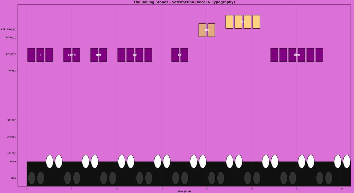
import matplotlib.pyplot as plt
import matplotlib.patches as patches
from matplotlib import colors

# ---------------------------------------------------------
# 1. 音楽データの定義(The Rolling Stones: Satisfaction Vocal)
# 形式: (開始X, ピッチ, オクターブ, 持続ブロック数, 歌詞テキスト)
# ---------------------------------------------------------
vocal_line = [
    (0,  6,   1, 3, "I"),         # I (B)
    (4,  6,   1, 2, "can't"),     # can't (B)
    (7,  6,   1, 2, "get"),       # get (B)
    (10, 6,   1, 4, "no"),        # no (B)

    (16, 6,   1, 2, "sa"),        # sa (B)
    (19, 0.5, 2, 2, "tis"),       # tis (C#)
    (22, 1,   2, 4, "fac"),       # fac (D)
    (27, 6,   1, 6, "tion")       # tion (B)
]

# ベースとドラムは伴奏・重力の基盤として継続
bass_line = []
for i in range(0, 38, 2):
    bass_line.append((i, 2, 0, 1))

drums = []
for i in range(0, 38, 4):
    drums.append((i, 98, 0, 2))
    drums.append((i+2, 99, 0, 2))

# ---------------------------------------------------------
# 2. 法則に基づく色の定義
# ---------------------------------------------------------
base_colors = {
    0.5: '#C45500',  # C# (ド#)
    1: '#FFA500',    # D (レ)
    2: '#FFFF00',    # E (ミ)
    6: '#800080',    # B (シ)
    98: '#333333',
    99: '#FFFFFF'
}

def get_color(pitch_class, octave):
    base_hex = base_colors.get(pitch_class, '#000000')
    base_rgb = colors.to_rgb(base_hex)
    if pitch_class >= 98: return base_rgb
    if octave <= 0: return [c * 0.4 for c in base_rgb]
    elif octave == 1: return base_rgb
    else:
        factor = 1.0 - (0.5 ** (octave - 1))
        return [c + (1.0 - c) * factor for c in base_rgb]

# ---------------------------------------------------------
# 3. 描画キャンバスの設定(正方形 + 指定の背景色)
# ---------------------------------------------------------
bg_color = '#da70d6' # 主調色(オーキッド)
text_color = '#1A1A1A'

fig, ax = plt.subplots(figsize=(12, 12))
fig.patch.set_facecolor(bg_color)
ax.set_facecolor(bg_color)

# 大地(ベース・ドラム層)
ax.add_patch(patches.Rectangle((0, -1), 40, 1.5, facecolor='#111111', edgecolor='none', zorder=1))

# ---------------------------------------------------------
# 4. ブロックを描画する関数(ボーカル用拡張)
# ---------------------------------------------------------
def draw_track(track_data, is_drum=False, is_vocal=False):
    for note in track_data:
        if is_vocal:
            start_x, pitch_class, octave, duration, lyric = note
        else:
            start_x, pitch_class, octave, duration = note

        if pitch_class == 98: y = -0.5
        elif pitch_class == 99: y = 0.5
        else: y = pitch_class + 1 + (octave - 1) * 7

        note_color = get_color(pitch_class, octave)

        # ブロック群の描画
        for i in range(duration):
            sq_x = start_x + i + 0.1
            sq_y = y - 0.45

            if is_drum:
                rect = patches.Circle((sq_x + 0.45, sq_y + 0.45), 0.4,
                                      facecolor=note_color, edgecolor='black', linewidth=1.5, zorder=3)
            else:
                rect = patches.Rectangle((sq_x, sq_y), 0.8, 0.8,
                                         facecolor=note_color, edgecolor='black', linewidth=1.5, zorder=4)
            ax.add_patch(rect)

        # ボーカルの場合はブロック群の中央に歌詞テキストを配置
        if is_vocal:
            center_x = start_x + (duration / 2)
            center_y = y - 0.05
            ax.text(center_x, center_y, lyric, ha='center', va='center',
                    fontsize=14, fontweight='bold', color='white', zorder=5)

draw_track(drums, is_drum=True)
draw_track(bass_line, is_drum=False)
draw_track(vocal_line, is_vocal=True)

# ---------------------------------------------------------
# 5. 見た目の調整と出力
# ---------------------------------------------------------
ax.set_xlim(-1, 36)
ax.set_ylim(-1, 10)

ax.set_yticks([-0.5, 0.5, 1, 2, 3, 6, 7, 8, 8.5])
yticklabels = ['Kick', 'Snare', '1F: C(ド)', '2F: D(レ)', '3F: E(ミ)', '7F: B(シ)',
               '8F: C(ド高)', '9F: D(レ高)', '9.5F: C#(ド#高)']
ax.set_yticklabels(yticklabels, color=text_color, fontweight='bold')

ax.tick_params(axis='x', colors=text_color)
ax.tick_params(axis='y', colors=text_color)

ax.set_xlabel("Time (Grid)", color=text_color, fontweight='bold')
ax.set_title("The Rolling Stones - Satisfaction (Vocal & Typography)", color=text_color, fontweight='bold', fontsize=16)

plt.grid(True, which='both', axis='x', linestyle=':', alpha=0.3, color=text_color, zorder=1)
plt.tight_layout()
plt.show()
Satisfaction — Drum Section of the Instrumental Break
This time, this is a visualization of drummer Charlie Watts's drum performance during the instrumental break.
The white and black circles at the bottom of the image represent the drum strikes.
◆The music is here.
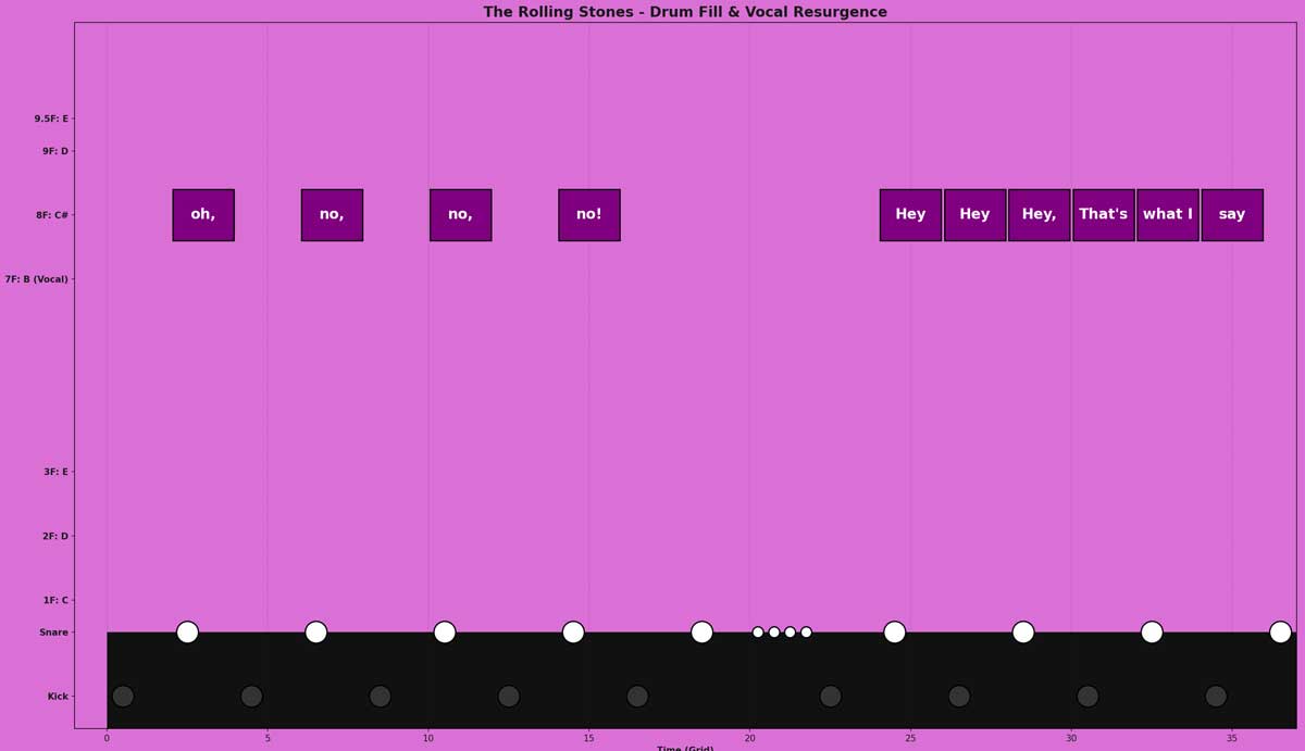
import matplotlib.pyplot as plt
import matplotlib.patches as patches
from matplotlib import colors

# ---------------------------------------------------------
# 1. 音楽データの定義("no, no, no" -> ドラムフィル -> "Hey, Hey")
# ---------------------------------------------------------
vocal_line = [
    # 前半 (感情の拒絶)
    (2,  6, 1, 2, "oh,"),
    (6,  6, 1, 2, "no,"),
    (10, 6, 1, 2, "no,"),
    (14, 6, 1, 2, "no!"),

    # 後半 (反逆の再開: He HEI HEI ThatS)
    (24, 6, 1, 2, "Hey"),
    (26, 6, 1, 2, "Hey"),
    (28, 6, 1, 2, "Hey,"),
    (30, 6, 1, 2, "That's"),
    (32, 6, 1, 2, "what I"),
    (34, 6, 1, 2, "say")
]

drums = []
# 前半のビート (KickとSnareの反復)
for i in range(0, 16, 4):
    drums.append((i, 98, 0, 1))      # Kick
    drums.append((i+2, 99, 0, 1))    # Snare

# ブレイク部分の正確なドラムフィル(ツン タン ツツツツ ツン タン)
drums.append((16, 98, 0, 1))      # ツン (Kick)
drums.append((18, 99, 0, 1))      # タン (Snare)

# ツツツツ (Snareの16分音符4連打。持続時間を0.5として定義)
drums.append((20,   99, 0, 0.5))
drums.append((20.5, 99, 0, 0.5))
drums.append((21,   99, 0, 0.5))
drums.append((21.5, 99, 0, 0.5))

drums.append((22, 98, 0, 1))      # ツン (Kick)
drums.append((24, 99, 0, 1))      # タン (Snare / Heyと同時にクラッシュ)

# 後半のビート再開
for i in range(26, 38, 4):
    drums.append((i, 98, 0, 1))      # Kick
    drums.append((i+2, 99, 0, 1))    # Snare

# ---------------------------------------------------------
# 2. 法則に基づく色の定義
# ---------------------------------------------------------
base_colors = {
    6: '#800080',    # B (シ): ボーカルの主調色
    98: '#333333',   # Kick (黒に近いグレー)
    99: '#FFFFFF'    # Snare (白)
}

def get_color(pitch_class, octave):
    base_hex = base_colors.get(pitch_class, '#000000')
    base_rgb = colors.to_rgb(base_hex)
    if pitch_class >= 98: return base_rgb
    if octave <= 0: return [c * 0.4 for c in base_rgb]
    else: return base_rgb

# ---------------------------------------------------------
# 3. 描画キャンバスの設定(正方形 + 指定の背景色)
# ---------------------------------------------------------
bg_color = '#da70d6'   # 主調色(オーキッド)
text_color = '#1A1A1A'

fig, ax = plt.subplots(figsize=(12, 12))
fig.patch.set_facecolor(bg_color)
ax.set_facecolor(bg_color)

# 大地(黒い基盤)
ax.add_patch(patches.Rectangle((0, -1), 40, 1.5, facecolor='#111111', edgecolor='none', zorder=1))

# ---------------------------------------------------------
# 4. ブロックと完全正円を描画する関数
# ---------------------------------------------------------
def draw_track(track_data, is_drum=False, is_vocal=False):
    for note in track_data:
        if is_vocal:
            start_x, pitch_class, octave, duration, lyric = note
        else:
            start_x, pitch_class, octave, duration = note

        if pitch_class == 98: y = -0.5
        elif pitch_class == 99: y = 0.5
        else: y = pitch_class + 1 + (octave - 1) * 7

        note_color = get_color(pitch_class, octave)

        if is_drum:
            # 円をキャンバスの比率に関わらず「絶対的な正円」にするためScatterマーカーを使用
            # ツツツツ(duration 0.5)の連打は面積(s)を小さくする
            marker_size = 600 if duration >= 1 else 150
            cx = start_x + (0.5 if duration >= 1 else 0.25)
            cy = y
            ax.scatter(cx, cy, s=marker_size, c=[note_color], edgecolors='black', linewidths=1.5, zorder=3)

        elif is_vocal:
            # 歌詞ブロックを繋がった1つのソリッドな長方形として描画
            rect_width = duration - 0.1
            sq_x = start_x + 0.05
            sq_y = y - 0.4

            rect = patches.Rectangle((sq_x, sq_y), rect_width, 0.8,
                                     facecolor=note_color, edgecolor='black', linewidth=1.5, zorder=4)
            ax.add_patch(rect)

            # テキストの中央配置
            center_x = start_x + (duration / 2)
            center_y = y
            ax.text(center_x, center_y, lyric, ha='center', va='center',
                    fontsize=16, fontweight='bold', color='white', zorder=5)

draw_track(drums, is_drum=True)
draw_track(vocal_line, is_vocal=True)

# ---------------------------------------------------------
# 5. 見た目の調整と出力
# ---------------------------------------------------------
ax.set_xlim(-1, 37)
ax.set_ylim(-1, 10)

ax.set_yticks([-0.5, 0.5, 1, 2, 3, 6, 7, 8, 8.5])
yticklabels = ['Kick', 'Snare', '1F: C', '2F: D', '3F: E', '7F: B (Vocal)',
               '8F: C#', '9F: D', '9.5F: E']
ax.set_yticklabels(yticklabels, color=text_color, fontweight='bold')

ax.tick_params(axis='x', colors=text_color)
ax.tick_params(axis='y', colors=text_color)

ax.set_xlabel("Time (Grid)", color=text_color, fontweight='bold')
ax.set_title("The Rolling Stones - Drum Fill & Vocal Resurgence", color=text_color, fontweight='bold', fontsize=16)

plt.grid(True, which='both', axis='x', linestyle=':', alpha=0.3, color=text_color, zorder=1)
plt.tight_layout()
plt.show()
Click here for other pages in this series!
■【PartⅡ Law for Translating Music into Painting 】— Examples of Paintings in Which Color Chords Are Actually Used: Ryuzaburo Umehara’s Mount Fuji!(梅原龍三郎 富士山)【Go to this page!】
■【PartⅢ Law for Translating Music into Painting 】The History of Previous Research on this Law and an Examination of the Innovation and Value of My Theory【Go to this page!】
■【PartⅣ Law for Translating Music into Painting】As a Symbol of the “300-Year-Old Problem of Being Unable to Create Forms” — Rimington’s Color Piano, Which Adopted the Spectrum Correspondence Table!
【Go to this page!】